From Raw Sensor Logs to an Activity Classifier

Why I built this

Activity recognition sits in a sweet spot for practical ML. The inputs are messy real-world signals, the labels are concrete, and the modeling decisions are easy to explain. You can start simple and still learn a lot about preprocessing discipline.

I used the WISDM dataset, which includes accelerometer and gyroscope streams from phones and watches. The task is multi-class classification: predict an activity code from motion patterns.

Stage 1: from raw files to usable tables

The first notebook, DataLoader.ipynb, does most of the heavy lifting for ingestion. It parses raw text files and ARFF feature files, tags rows by device and sensor type, and exports two main tables: raw.csv and arff.csv.

This step looks boring on paper, but it decides everything that comes later. If naming, timestamps, or column types are even slightly inconsistent here, model quality drops and debugging gets painful.

Stage 2: preprocessing and sensor fusion

In PhoneXGB2.ipynb, I convert x/y/z to numeric values, parse timestamps, one-hot encode sensor metadata, and scale accelerometer and gyroscope channels separately.

The key decision was to train a phone-only pipeline first and merge phone accelerometer and gyroscope streams on shared keys: timestamp, subject id, and activity code. Keeping that merge explicit made errors easier to catch.

# Merge accel + gyro streams after cleaning
phone_accel = df[(df["Device"] == "phone") & (df["Sensor"] == "accel")]
phone_gyro = df[(df["Device"] == "phone") & (df["Sensor"] == "gyro")]

merged = phone_accel.merge(
    phone_gyro,
    on=["Timestamp", "Subject-id", "Activity Code"],
    suffixes=("_acc", "_gyro")
)

# Features per timestep: 6 channels (3 accel + 3 gyro)
X = merged[["x_acc", "y_acc", "z_acc", "x_gyro", "y_gyro", "z_gyro"]].values

Stage 3: windowing time series for XGBoost

Raw sensor rows are not ideal for classification directly, so I frame them into sliding windows. I used frame_size=80 and hop_size=40, then flattened each (80, 6) window into a tabular feature vector.

I ended up with 72,727 framed samples. At that point I had two choices: sequence models or tree models. I went with XGBoost first because I wanted a hard baseline I could iterate quickly and inspect class by class before reaching for deeper architectures.

def create_windows(features, labels, frame_size=80, hop_size=40):
    X_windows, y_windows = [], []
    for i in range(0, len(features) - frame_size, hop_size):
        window = features[i:i + frame_size]
        segment_labels = labels[i:i + frame_size]
        label = np.bincount(segment_labels).argmax()  # majority label in the frame
        X_windows.append(window)
        y_windows.append(label)
    return np.array(X_windows), np.array(y_windows)

Xw, yw = create_windows(X, y)
Xw_flat = Xw.reshape(Xw.shape[0], -1)  # flatten for XGBoost

Stage 4: training and evaluation

This is where most of my effort went. XGBoost was not a side detail in this project. It was the center of the whole pipeline once framing and fusion were stable. I split the framed data 80/20 (58,181 train and14,546 test), flattened the windows, and trained with my best random-search parameter set.

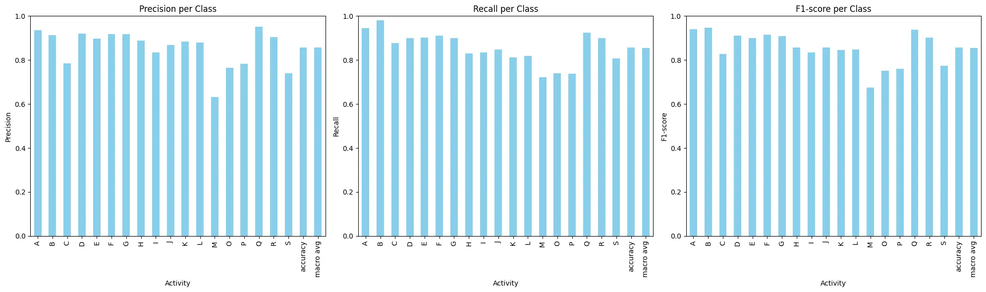
The best run reached0.855905 accuracy. More important than that single number was the class-level behavior. Some classes were very strong and some were consistently noisy, and the confusion matrix made it obvious where.

xgb_model = xgb.XGBClassifier(
    use_label_encoder=False,
    eval_metric="mlogloss",
    colsample_bytree=0.9396893641976711,
    gamma=0,
    learning_rate=0.10241823755571676,
    max_depth=6,
    n_estimators=982,
    subsample=0.8545330472743582,
    device="cuda",
    early_stopping_rounds=10
)

xgb_model.fit(X_train, y_train, eval_set=[(X_test, y_test)], verbose=False)
y_pred = xgb_model.predict(X_test)
accuracy = accuracy_score(y_test, y_pred)

The standout classes were sitting, writing, and standing. The weaker ones were jogging, stairs, kicking, and dribbling. That lines up with intuition: classes with similar motion profiles overlap more in the feature space.

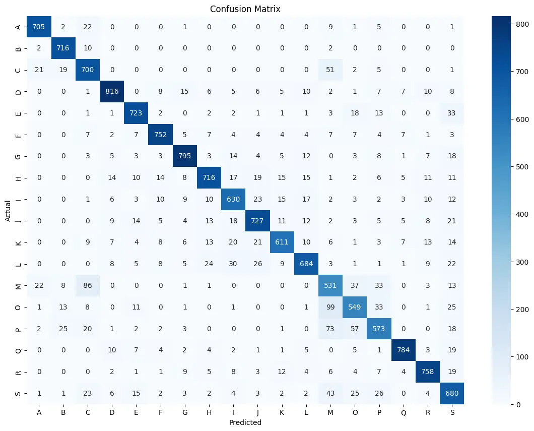
• Strong classes: D (sitting), Q (writing), E (standing).
• Weak classes: B (jogging), C (stairs), M (kicking), P (dribbling).
• Repeated confusions: A↔B/C and some G/H↔E overlap.

I also hit a practical training warning: device mismatch (GPU booster but CPU input matrix), which still runs but adds overhead. So even when the metric looked good, there was still systems-level cleanup left to do.

What was harder than expected

• Scale and memory pressure. The raw data is large enough that one careless dataframe copy can slow the entire notebook loop.
• Environment mismatch warnings. XGBoost showed CPU/GPU mismatch warnings in some runs. It still worked, but with unnecessary overhead.

What I learned

The model choice mattered, but the biggest gains came from cleaning and alignment choices upstream. In sensor projects, strong preprocessing is not optional. It is most of the work.

I also stopped trusting aggregate metrics alone. A confusion matrix tells you where the model is genuinely useful and where it is still guessing between similar activities.

What I would improve next

Wrapping up

This project gave me exactly what I wanted: a practical pipeline that works, plus a list of concrete next moves. The classifier is useful already, and the failure modes are clear enough to improve without guesswork.

If you are building from wearable or phone sensor data, start with your preprocessing story. Once that is solid, model iteration gets much faster.