Teaching a Car to Park by Imagining the Future, and Learning When Not to Trust It

A planner can look intelligent because every future it considers is perfectly simulated. With the real vehicle physics, it can test action sequences, rewind, and choose a move toward the stall. The search is real, but the imagination is an oracle.

Replace that oracle with a learned model and every candidate future becomes a prediction. One-step errors can feed the next prediction until the planner optimizes a future the real car never visits. The model can be confidently wrong: low training loss, goalward predicted latents, and a quiet uncertainty heuristic while the car misses.

This project builds that entire chain in a deliberately small setting: the kinematic parking-v0 environment, a cross-entropy method optimizer, observation-space dynamics models, a joint-embedding predictive architecture, latent-space planning, and three practical distrust signals. The most useful result is not a parking demo. It is the separation between three questions that are easy to blur:

1. Can the optimizer reach the environment outcome when its model is correct?
2. Can a learned representation predict held-out transitions better than a trivial baseline?
3. Can the controller park, and can its alarm detect when it is about to fail?

The answers were yes, yes, and no.

TL;DR

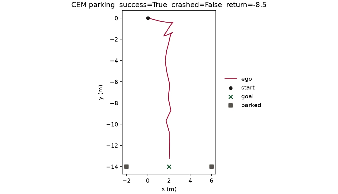
• True-dynamics CEM reaches the environment's success diagnostic, then a scripted brake finishes the tape. CEM controls the first 40 actions through the success-triggering action. That loose flag fires about 3.9 m from the goal at about 4.5 m/s; the reward weights lateral/y error cheaply and ignores speed. Five scripted full-brake actions [-1, 0] then cross the recorder's separate stop condition and finish about 1.8 m away at 0.5 m/s. The stopped pose is not entirely CEM output.
• Learned latent MPC, meaning MPC that scores imagined futures from a learned latent predictor, parks 0 of 6 measured seeds. In the recorded six-seed run, one episode crashed and five reached the duration cutoff. For seed 0, receding latent MPC reached a best xy distance of 20.0 m before crashing at step 315. Open-loop latent control reached 9.4 m before crashing at step 415. Neither set info["is_success"].
• The tested distrust signals perform at chance on crash-soon detection. The positive class contains only 10 of 2,815 finite disagreement rows, so chance precision is approximately 0.004. Residual, one-step ensemble disagreement, and imagined horizon spread do not rise usefully above that line. A p90 disagreement cutoff of approximately 0.027 has precision 0 and recall 0 on the completed diagnostic tapes.

The true-dynamics numbers are recalculated from saved arrays. Several latent-control and gate numbers come from lab notes and plot titles because raw per-step arrays were not retained.

The experiment

The environment is Farama's parking-v0, used through the Gymnasium environment API. It is a compact bicycle-style simulator, not a camera pipeline and not a 3D driving stack. Pixels were never trained. That keeps the experiment focused on planning and model error rather than perception.

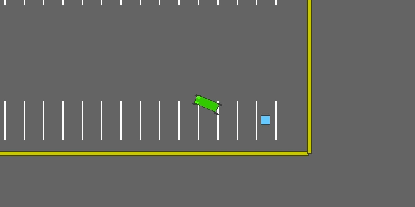
At reset, the installed environment returns a dictionary with three keys:

observation
achieved_goal
desired_goal

Each value has six features in this order:

[x, y, vx, vy, cos_h, sin_h]

The first two numbers are position, the next two are velocity, and the final pair is heading represented by cosine and sine. The continuous action is exactly [acceleration, steering], with both components in [-1, 1]. The highway-env action documentation calls the first component throttle; the local data names it acceleration.

The stored coordinates are scaled. The configured scale vector is [100, 100, 5, 5, 1, 1], and the installed implementation divides all three dictionary vectors, observation, achieved_goal, and desired_goal, by it. Stored x and y are physical metres divided by 100. Stored vx and vy are physical metres per second divided by 5. Heading is unchanged. This still occurs even though the configuration says normalize=False, so treating stored x as metres would make every model metric misleading.

The simulator advances physics at 15 Hz and accepts policy actions at 5 Hz. Each action therefore covers 0.2 seconds and contains three physics frames. A planning horizon of ten actions covers two seconds.

Four outcome fields need careful names. In the normal environment, terminated means that the task ended because of a crash or because every controlled agent met the environment's success test. truncated means the configured 100-second duration was reached. info["crashed"] identifies collision, while info["is_success"] separately identifies whether the goal criterion is met. Visual closeness is not a substitute for that success diagnostic.

For more detail on these fields, see lesson 0001, the parking-v0 reference, and the project glossary.

First, prove the planner can work

Before learning a model, the project tests the optimizer in two increasingly relevant settings.

The first is Gymnasium's Pendulum-v1. CEM proposes action sequences, the true Pendulum simulator evaluates them, and the controller repeatedly executes one action and replans. In the saved check, CEM return is -125.7, compared with -1071.9 for random control.

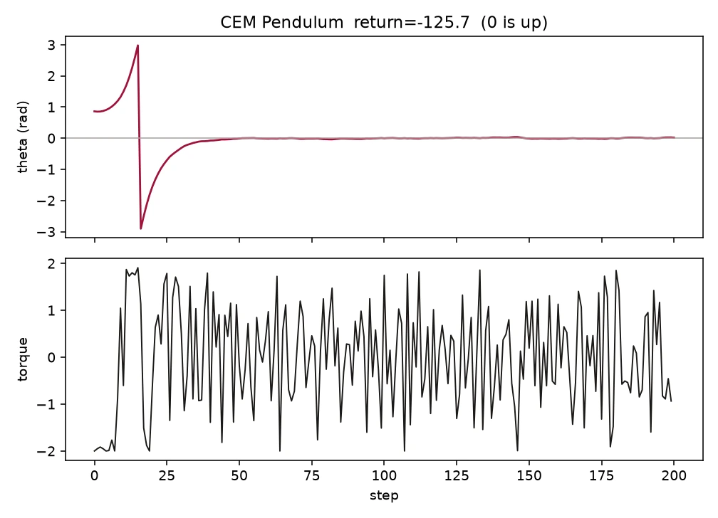
That boundary is important. Pendulum has different dynamics, observations, rewards, constraints, and geometry. It can reveal a broken optimizer, but it cannot validate parking behavior.

The second check uses parking-v0 itself and lets scripts/plan_parking.py imagine with the true simulator. For every candidate action sequence, the planner copies the simulator, calls its real step function through the horizon, accumulates cost, and restores the copied state in a finally block. Source inspection shows that the snapshot covers ego pose, speed, action and collision fields, environment counters, the action type's last action, road-object collision fields, and all vehicle states. A rewind self-check confirms that imagined evaluation does not move the real ego or neighboring vehicles and restores timing and collision state.

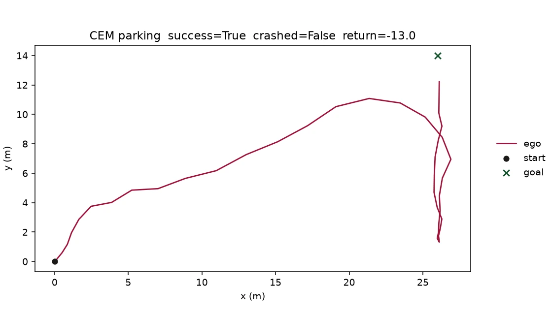
The tape contains 45 real transitions. CEM supplies actions 1 through 40, including the success-triggering action on zero-based row 39. At that point the car is about 3.9 m from the goal and moving about 4.5 m/s. The loose diagnostic fires because the reward weights lateral/y error at 0.3 versus x at 1 and ignores speed, which motivates continuing the recording.

Recording mode replaces normal success termination with crash-only termination, then sends scripted full brake [-1, 0] for the final five actions. The six true success rows are repeated flags in one trajectory, and saved terminated stays false. The recorder stops when its separate condition, under 1.8 m and 0.6 m/s, is crossed: the saved final pose is about 1.8 m and 0.5 m/s, with tape return about -13.0. That stop condition is not an independent parking-quality threshold, and the final pose is not entirely CEM output. Report both necessary checks: environment outcome and physical finishing pose.

The same true-dynamics planner was then stressed by placing parked cars in neighboring stalls. Those obstacles remain hidden from the default six-feature observation. CEM reacts to them only because candidate rollouts can physically collide in the copied simulator.

The runs take 48 and 39 real steps respectively. They show that the optimizer and simulator-rewind machinery can find collision-aware action sequences in these two constructed cases. They do not show that the learned model represents neighboring cars, because those cars are not present in its default observation.

CEM: guess, keep, refit

The cross-entropy method, as applied to real-time planning by Pinneri et al., optimizes complete action sequences. Let the horizon be $H$, the action dimension be $A=2$, and a candidate sequence be $u_{1:H}\in\mathbb{R}^{H\times A}$. CEM maintains a diagonal Gaussian with a mean and standard deviation for every time and action coordinate.

The repository's core loop is short:

samples = np.clip(mean + std * noise, low, high)
elite_idx = np.argpartition(costs, n_elites - 1)[:n_elites]
elites = samples[elite_idx]
mean = elites.mean(axis=0)
std = np.maximum(elites.std(axis=0), 1e-6)

First, sample many tapes from the current Gaussian and clip every action to the legal range. Next, evaluate a cost for each tape. Keep the $K$ lowest-cost tapes, called elites, then refit the Gaussian to their population mean and population standard deviation. Repeat that refinement several times.

The implementation also retains the best actually scored elite seen across all iterations. It executes the first action of that best scored sequence, not the fitted Gaussian mean. On the next real step, a warm start drops the committed action, shifts the rest left, and repeats the final action.

That makes this a small CEM-MPC variant with clipped Gaussian sampling, lowest-cost elite refitting, best-scored-action execution, and a warm start. It differs from Pinneri et al.'s vanilla pseudocode, which does not combine clipping with best-sequence execution. The precise local loop is more informative than a broad variant label.

For true-dynamics parking, scripts/plan_parking.py uses horizon 10, 24 samples, 6 elites, and 3 refinement iterations by default. Cost is negative accumulated reward plus a remainder penalty after an imagined crash, preventing an early collision from becoming cheap merely because it ends evaluation.

Receding horizon: imagine ten, execute one

CEM answers, "Which action tape is cheapest under this model?" Model-predictive control, or MPC, answers, "How do I repeatedly use that optimizer while the real system changes?"

At real time $t$, the receding-horizon loop is:

1. Read the current real observation $o_t$.
2. Optimize $H=10$ imagined actions.
3. Execute only the first action of the best scored tape.
4. Receive the real next observation $o_{t+1}$.
5. Shift the previous tape as a warm start and optimize again.

The controller imagines ten actions but commits one. This distinction limits how long it runs blind. A bad prediction at the end of a two-second horizon does not directly force ten real actions. After 0.2 seconds, the controller sees reality again.

Replanning does not erase model error, however. The optimizer can still exploit the learned model inside each horizon. If the model consistently assigns low cost or low planning energy to physically bad tapes, replanning produces a fresh bad tape from every new observation. MPC contains open-loop error; it does not make an inaccurate model accurate.

The true-dynamics run separates two checks: CEM reaches the environment outcome with the real bicycle, and scripted braking reaches the recorder's finishing pose. The next experiment replaces that imagination.

See lesson 0002, the CEM-MPC reference, and scripts/cem.py for the executable details.

Turn driving into transitions

A learned dynamics model needs examples of what one action does. Each example is a transition:

Here $o_t$ is the current six-feature observation, $a_t$ is [acceleration, steering], and $o_{t+1}$ is the real next observation returned by the environment. The saved row also includes reward, achieved and desired goals, episode ID, and outcome flags.

scripts/collect_random.py gathered exactly 8,000 random-policy transitions. They span 92 represented episode IDs because collection stopped partway through the last episode. Among 91 completed episodes, zero completed successfully, all 91 crashed, and none reached the duration cutoff. There are zero success flags anywhere in that file.

The training mix in scripts/train_dynamics.py adds one 45-transition true-dynamics CEM trajectory. It is the only successful parking trajectory in the training mix and is forced into the training side rather than validation. The remaining episodes are split 80/20 by episode ID.

Splitting by episode matters. Adjacent rows from one trajectory are strongly related: the next observation in row $t$ is the current observation in row $t+1$. A random row split would place near-duplicates on both sides and make validation look more independent than it is. An episode-level split keeps each random trajectory entirely in training or validation.

The dataset is therefore not balanced experience from a competent driver. It is almost entirely random wandering and crashes, plus one successful tape. That fact is an observation about the file. Whether more successful or corrective data would fix latent planning is a hypothesis, not something this experiment isolates.

Beat the prediction that nothing changes

Before judging a learned model, define a baseline that can win whenever adjacent observations barely move. The identity predictor ignores the action and says:

scripts/identity_baseline.py implements this equation by subtracting $o_t$ from $o_{t+1}$, squaring elementwise, and taking the mean.

Its overall one-step mean squared error on the random dataset, in stored coordinates, is approximately 0.0033. This number is small partly because one policy step is only 0.2 seconds and partly because position is divided by 100. The feature-level errors make the scale visible.

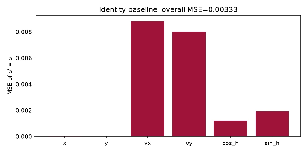
The recalculated feature MSEs, rounded for reporting, are 0.0000193 for x, 0.0000129 for y, 0.00881 for vx, 0.00801 for vy, 0.00122 for cos_h, and 0.00190 for sin_h. These are stored-coordinate errors, not metres or metres per second.

Let $f$ be the observation-space world model. It receives the current observation and action and predicts the next selected observation features:

If a batch has $B$ transitions and the output has $D$ features, training uses elementwise mean squared error:

scripts/train_dynamics.py implements the direct prediction in DynamicsMLP.forward and the elementwise mean in train_model with default-mean F.mse_loss.

The model predicts the next observation directly, not a delta. Its one-step validation loss needs to beat identity before its horizon curve is interesting. Calling this metric accuracy would be wrong because it is a continuous regression error.

Pose is not the full state

The full model predicts all six features. Two reduced alternatives ask whether position and heading alone are enough:

• A pose-only model uses $x,y,\cos h,\sin h$.
• A stacked-pose model concatenates the two latest poses, using their difference as an indirect clue about motion.

To compare these models fairly, the evaluation reports pose MSE for all of them. Comparing the full model's six-output MSE against a four-output model's overall MSE would mix model quality with a change in denominator and would remove the relatively large velocity terms. Pose MSE evaluates the shared coordinates only.

The conceptual issue is the Markov property. A state is Markov when the next state depends on the latest state and action, not on unobserved history. Two cars can have the same pose while moving at different velocities. Give both the same acceleration and steering, and their next positions differ. Pose alone is therefore a partially observed view of the bicycle dynamics.

The two-pose stack tries to infer velocity from recent change. In these stored units, however, position differences over 0.2 seconds are tiny because metres are divided by 100. A shallow MLP must extract that weak signal while also learning the dynamics. In this run, stacking does not solve the long-horizon problem.

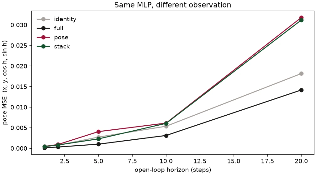
At horizon one, every model receives a real validation observation. At horizon two, its first prediction becomes its next input. This continues through horizons 5, 10, and 20. The plot therefore measures repeated self-feeding, not twenty independent one-step predictions.

The full model's better curve supports a narrow conclusion: exposing velocity improves open-loop pose prediction on these held-out starts. It does not prove that six features are a complete state for every parking configuration. In the neighboring-car stress test, for example, the observation omits the obstacles.

See lesson 0004 and the partial-observation reference for a visual treatment.

One good step can become a bad future

One-step MSE averages local predictions near data the model has seen. Planning asks a harsher question. The model must consume its own outputs, often under action sequences selected precisely because they look attractive to that model.

The next figure replays the saved tape through three observation-space models without revealing the real trajectory again: imagined full uses all six features, imagined pose uses pose only, and imagined stack uses two poses.

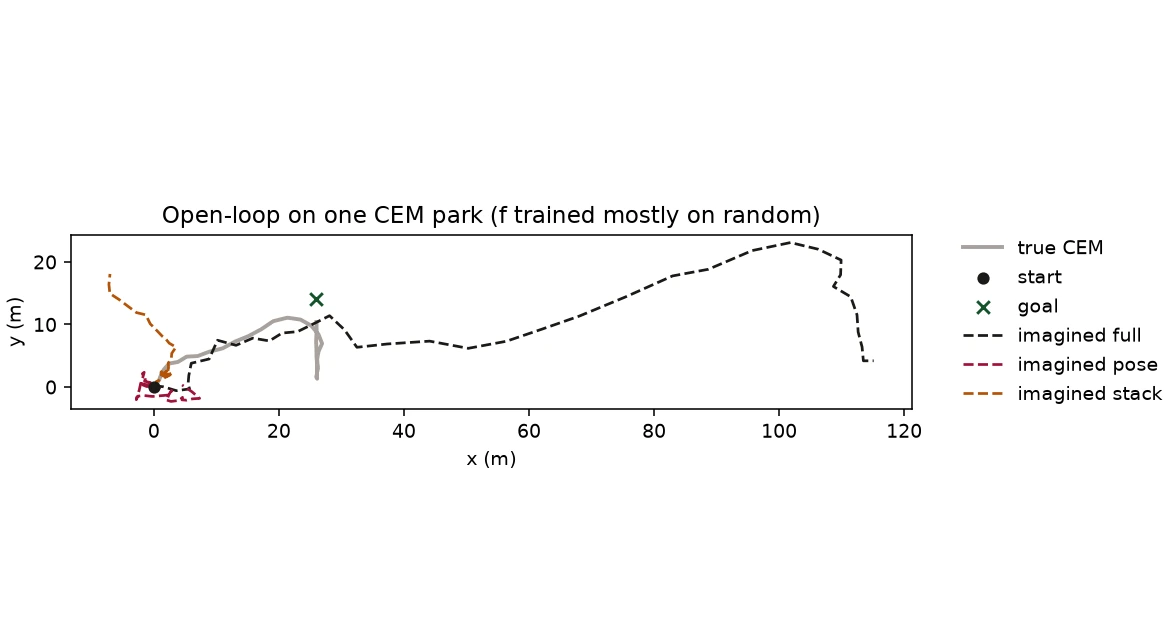
This is compounding error: a one-step prediction lands off the real data manifold, then becomes the next synthetic input, so drift can accelerate. Nagabandi et al.'s model-based control work makes the same distinction between one-step fit and multi-step rollout.

MPC reduces exposure by replanning from the current real observation after each committed action. Still, every CEM candidate is ranked using an open-loop rollout inside the horizon. If that rollout is untrustworthy, the optimizer is choosing actions with a distorted ruler.

This gives a stronger baseline for the latent model: do not ask only whether its next-step loss is low. Ask whether its open-loop error remains below a meaningful identity baseline across the planning horizon, then separately ask whether the resulting controller parks.

Predict a latent, not the snapshot

Unweighted MSE applies equal loss weight to each stored coordinate, even though those coordinates differ in physical scale and task importance. A joint-embedding predictive architecture, or JEPA, instead learns a latent space in which prediction is trained.

Define the symbols before the equations:

• $o_t$ is the current real observation.
• $a_t$ is the current action.
• $E$ is the online encoder with parameters $\theta_{\text{online}}$.
• $E_{\text{target}}$ is a slowly updated target encoder with parameters $\theta_{\text{target}}$.
• $z_t$ is the online latent for the current observation.
• $z^*_{t+1}$ is the target latent for the real next observation.
• $P$ is the latent predictor.
• $\hat z_{t+1}$ is its predicted next latent.

The forward equations are:

For batch size $B$ and latent dimension $D_z$, the repository trains with mean squared latent error:

The local architecture uses small MLPs on six-dimensional kinematics and an eight-dimensional latent. It is not an image JEPA, video model, transformer, autoencoder, or pixel generator. There is no decoder. The closest conceptual connection to I-JEPA is the online encoder, predictor, slow target encoder, and prediction in representation space. The exact local objective is established by scripts/train_jepa.py.

Keep the target from chasing the guess

If both sides of the loss learn freely from the same gradient, they can make the task easy in an unhelpful way. The target could move toward whatever the predictor already outputs. This implementation prevents that in two ways.

First, target encoding runs under torch.no_grad(), target parameters have requires_grad=False, and they are excluded from the optimizer. That is the stop-gradient boundary. Calling .eval() would not be sufficient: evaluation mode changes dropout and batch-normalization behavior, but it does not detach tensors or disable autograd.

Second, the target parameters follow the online encoder using an exponential moving average. Let $\tau=0.99$ be the target retention coefficient. After an online update:

The Jepa.ema_ method in scripts/train_jepa.py performs this update under torch.no_grad().

The target moves slowly, giving the predictor a stable answer key without freezing that answer key forever. A focused version of the training loop is:

z_hat = model.predict(model.encode(o), a)
z_tgt = model.encode(o2, target=True)
loss = F.mse_loss(z_hat, z_tgt)
loss.backward()
optimizer.step()
model.ema_(tau=0.99)

In the actual class, target encoding supplies the no-gradient context. The excerpt shows the data flow, not every safety line.

Check for collapse

A decoder-free latent objective has a dangerous trivial solution: map every observation to the same vector. Then predicting the next latent is easy because every answer is identical. Low loss alone cannot rule this out.

Before writing the horizon plot, the training script checks target latents from strided validation observations using two simple statistics:

1. Mean of the per-dimension latent sample standard deviations.
2. Mean off-diagonal pairwise Euclidean distance for up to 128 target latents.

scripts/train_jepa.py exits if either statistic is below 0.001. For the saved checkpoint, recalculation on 1,670 validation rows gives mean per-dimension standard deviation 1.0237 and mean pairwise distance 3.4962. Both pass the implemented threshold.

These checks rule out a near-constant target representation under two basic tests; they do not prove control usefulness.

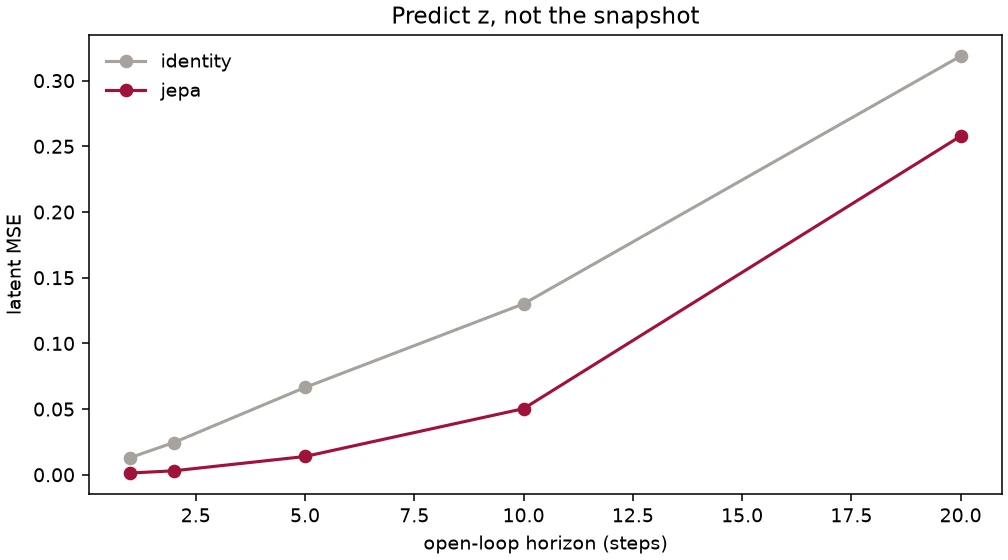
Latent identity keeps the current target encoding fixed while the real target latents genuinely move across each window. JEPA beating that baseline is therefore informative about temporal prediction, but it does not validate latent distance as a control objective.

See lesson 0005 and the JEPA reference.

Put CEM inside the learned imagination

The latent controller preserves the optimizer and receding-horizon shape from the true-dynamics experiment. It changes two things: candidate futures are rolled through $P$, and cost is distance to a goal latent.

Define $g$ as the desired-goal vector from the observation dictionary. The target encoder produces the goal embedding:

At real step $t$, planning starts from $z_t=E(o_t)$. For candidate actions $a_{t:t+H-1}$, recursively define each imagined latent:

The default planning energy is the sum of Euclidean distances to the goal latent across all predicted future steps:

scripts/plan_latent.py minimizes this energy with CEM using 64 samples, 8 elites, and 5 refinement iterations by default. The receding controller executes best[0], receives the next real observation, and repeats. A focused version of the planning loop is:

for h in range(horizon):
    z = model.predict(z, actions[:, h])
    energy += torch.linalg.vector_norm(z - z_goal, dim=-1)

Planning energy is latent distance, not the JEPA training loss, physical metres, or environment reward. In the recorded seed-0 run, it is near 3.5 while the car remains about 20 m from the stall.

V-JEPA 2 is related because it uses goal representations, CEM, and receding replanning. Its video representations, terminal L1 energy, and fitted-mean action differ from this project's summed per-step L2 and best-scored tape. Local --terminal remains final-step L2.

TD-MPC2 is another decoder-free latent planning reference, but it also learns reward, terminal value, and a policy prior and uses a different planner. The shared idea is local planning in learned latent dynamics, not architecture or performance equivalence.

The recorded comparison is sobering:

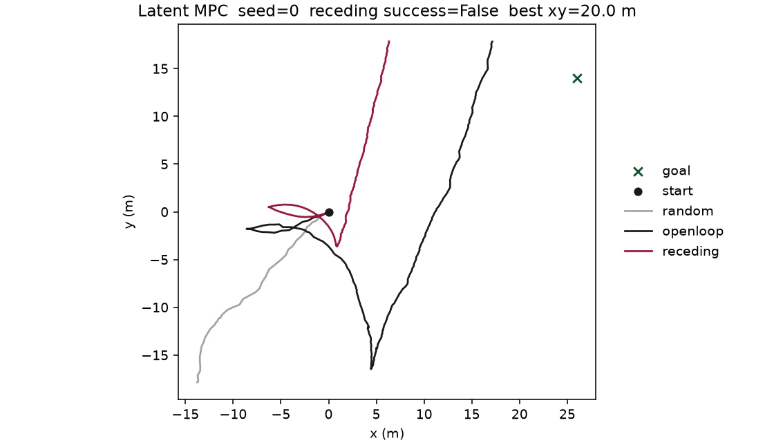
Recorded seed 0: random control crashes at step 53 after best xy 29.5 m; receding latent MPC reaches 20.0 m and crashes at step 315; open-loop reaches 9.4 m and crashes at step 415. Here open-loop commits one $H$-action tape before replanning, not one tape for the whole episode.

None parks because none sets info["is_success"]; closeness is secondary.

The recorded six-seed receding run has zero successes, one crash, and five duration cutoffs, so it parks 0 of 6 measured seeds. These values come from lab notes and plots, not saved raw arrays.

See lesson 0006 and the latent MPC reference.

Can the model notice when its future is unreliable?

A failed learned planner is easier to deploy safely if it can abstain before a dangerous action. The project tests three heuristics:

They answer different questions at different times. Residual grades the step that just happened. Disagreement and imagined spread estimate uncertainty about a proposed action or tape before it is sent.

The ensemble consists of three deterministic predictors sharing frozen online and target encoders. Each predictor is trained on a different bootstrap resample of the training transitions. This is not the probabilistic ensemble and trajectory-sampling architecture in PETS. PETS is useful background for model ensembles; it is not an equivalence claim.

Residual: grade the step after taking it

Let the one-step prediction be $P(E(o_t),a_t)$, and let the answer key after the real transition be $E_{\text{target}}(o_{t+1})$. The residual is one Euclidean norm:

scripts/plan_latent.py implements this equation in one_step_residual, using one L2 norm after the real step and no gradient tracking.

It is not a mean squared error and not an average over an episode. Because $o_{t+1}$ does not exist until env.step(a_t) returns, $r_t$ arrives after action $a_t$. A residual gate can prevent action $a_{t+1}$, but it cannot undo action $a_t$.

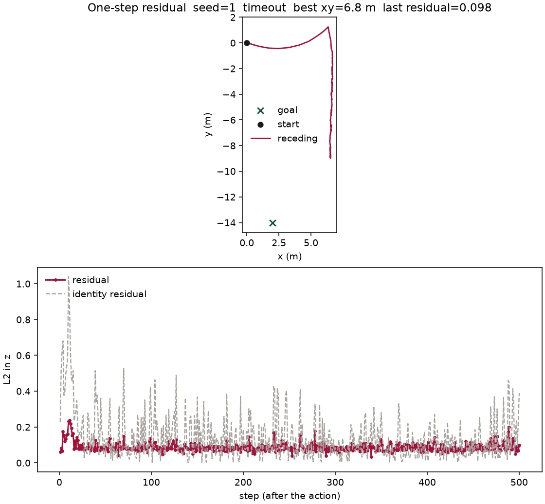
This seed-1 trace rejects a tempting inference: a quiet one-step residual does not imply a successful plan. The model can track ordinary local motion while its goal geometry or long rollouts remain unsuitable for control.

Residual also mixes two effects. It can rise because the action reaches unfamiliar physical behavior, or because the encoder makes nearby observations far apart in latent space. Without calibration against outcomes, magnitude alone is not a warning threshold.

Disagreement: ask several predictors before acting

For three predictors $P_i$, compute each next-latent guess from the same current latent and proposed action. Let $\operatorname{Std}_{\text{pop}}$ mean population standard deviation across ensemble members, computed separately for each latent dimension. One-step disagreement is:

scripts/plan_latent.py implements this equation in ensemble_disagreement with unbiased=False, followed by one L2 norm, all before env.step.

The inner operation produces one standard deviation per latent coordinate. The outer L2 norm reduces that vector to one scalar. The implementation uses unbiased=False, so this is population rather than sample standard deviation.

Imagined spread uses the same reduction after every predictor rolls its own latent through the planned horizon. It is available before acting because it needs only the current latent, candidate tape, and predictors. In principle it can expose futures where model errors branch even if one-step guesses agree.

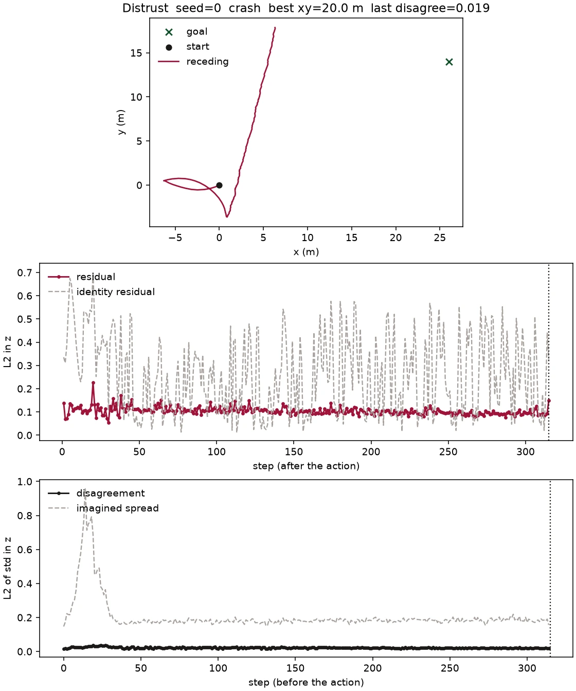
For this recorded seed-0 run, residual is about 0.107 early and 0.092 over the last ten steps, often below identity.

Agreement is not truth. Bootstrap predictors trained on the same narrow data and sharing the same encoder can inherit the same blind spot. If all three extrapolate similarly, disagreement stays low while all are wrong. Conversely, a spread spike can occur in an unfamiliar but harmless region. An uncertainty score becomes a detector only after its relationship to the event of interest is measured.

Precision and recall: did the alarm fire in time?

The event of interest is "a crash will occur within one planning horizon." With horizon $H=10$, action index $t$ receives a positive label when the actual crash action lies in indices $t$ through $t+9$. For one 315-step crashed tape, exactly its final ten pre-action positions are positive. Non-crashed tapes contain no positive crash-soon positions.

For a threshold $\gamma$, the alarm fires when a score is at least $\gamma$. Precision asks:

Recall asks:

These ratios apply when denominators are nonzero. In scripts/residual.py, crash_soon_labels creates labels and lagged_residual_scores aligns each previous-step residual to the next proposed action. pr_curve uses max(denominator, 1) defensively for empty cases; that safeguard does not affect this dataset.

In the recorded six-run diagnostic set, there are only 10 positive disagreement rows among 2,815 finite pre-action disagreement rows. The positive prevalence is:

That prevalence is chance precision for random alarms. The class imbalance is extreme because five runs do not crash and the one crash contributes only ten positive positions. A method can achieve high numerical accuracy by predicting "no crash soon" everywhere, which is why accuracy is not used here. Precision-recall curves focus on the rare positive event.

Lagged residual has one unavailable score at the start of each of six episodes, so its finite denominator is 2,809. The 10 / 2815 denominator specifically describes finite disagreement samples pooled over the same completed, non-aborted tapes.

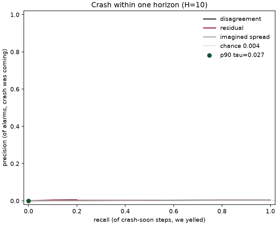
At the p90 disagreement threshold, approximately 0.027, observed precision and recall are both 0 on the completed diagnostic tapes.

The code can still wire that threshold into an abort:

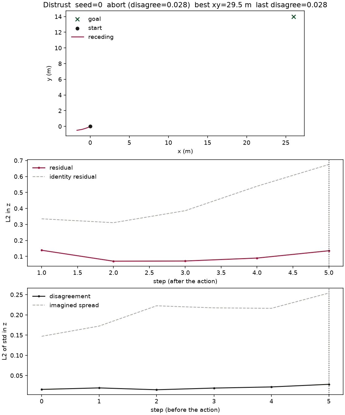
This is not a caught crash: the completed seed-0 tape crashes at step 315. The abort proves pre-action stopping, not useful detection.

See lesson 0007, the distrust reference, and scripts/residual.py.

Why did the learned planner fail?

The experiment supports several observations:

1. The random file has exactly 8,000 transitions and zero successful completed episodes among 91 completed episodes.
2. One true-dynamics 45-step parking trajectory is mixed into training and forced onto the training side.
3. The full observation model beats pose-reduced alternatives and identity on the reported prediction comparison, yet its replay of the successful CEM tape eventually diverges badly.
4. JEPA beats latent identity through horizon 20 on shared validation starts and passes the implemented non-collapse checks.
5. Learned latent MPC records zero successes in six measured seeds.
6. Planning energy can be low while physical distance remains large, because planning energy is latent distance, not metres or environment success.
7. The three tested distrust scores remain at chance for the recorded crash-soon labels.

Those observations do not isolate one causal failure. Several explanations are plausible.

Each paragraph above says "may" because the project did not vary one factor at a time. It would be an overclaim to say sparse successful data caused the failure, or that multi-step training would fix it. The current evidence narrows the debugging space without identifying a single cause.

What this project actually established

The project establishes an end-to-end experimental scaffold for model-based control:

• True-dynamics CEM reaches the environment outcome; scripted braking supplies the empty-lot recorder's final pose.
• Simulator snapshot and rewind separate imagined candidate steps from real committed steps.
• Saved transitions preserve action order, coordinate scales, goals, episode identity, and outcome flags.
• Episode-level splitting avoids placing adjacent rows from one random episode on both sides of train and validation.
• Identity is a necessary baseline because short, scaled transitions can produce deceptively small errors.
• Velocity matters for this bicycle's open-loop pose prediction.
• A decoder-free JEPA can pass simple non-collapse checks and beat latent identity without producing successful latent control.
• Residual timing differs fundamentally from disagreement timing: residual is post-action; disagreement and imagined spread are pre-action.
• A working abort mechanism is not a working detector. Detection must be scored against time-aligned outcomes under class imbalance.

It does not establish robust parking, safe autonomy, visual control, calibrated uncertainty, a V-JEPA 2 reproduction, a TD-MPC2 reproduction, or parity with probabilistic ensemble methods. It tests tiny MLPs on kinematic observations in one simulator.

The broad lesson is that prediction, planning, and distrust need separate acceptance tests. A horizon curve is not a park. A low planning energy is not a metre measurement. A threshold crossing is not a caught crash. Keeping those interfaces explicit makes a negative control result useful rather than ambiguous.

For a diagram connecting every component and figure, open lesson 0008 and the plot catalog.

What I would try next

The next experiments should isolate hypotheses instead of adding architecture at random.

The key comparison remains unchanged: first prove the optimizer with true dynamics, then replace only the imagination, then measure both task success and alarm quality.

Reproduce the experiment

Use Python 3.11 or newer. On Windows Git Bash, use .venv/Scripts/python if activation is inconvenient. From the repository root:

python -m venv .venv
source .venv/Scripts/activate
pip install -r requirements.txt
python scripts/sanity_check.py

Then reproduce in the documented dependency order:

python scripts/collect_random.py
python scripts/identity_baseline.py
python scripts/plan_pendulum.py
python scripts/plan_parking.py --record
python scripts/train_dynamics.py
python scripts/train_jepa.py
python scripts/plan_latent.py --compare --episodes 6
python scripts/train_ensemble.py
python scripts/residual.py --seed 1 --skip-check
python scripts/residual.py --gate --episodes 6 --skip-check

The ordering is functional. Random data precedes baseline and training. True-dynamics parking adds the successful tape before dynamics and JEPA training. JEPA precedes latent planning. The ensemble depends on the trained JEPA, and the gate depends on both.

The exact scripts are sanity_check.py, collect_random.py, identity_baseline.py, plan_pendulum.py, plan_parking.py, train_dynamics.py, train_jepa.py, plan_latent.py, train_ensemble.py, and residual.py.

Data and checkpoints are gitignored. Reproducing the stochastic learned-planner figures may require the recorded seeds and the same software environment. The saved true-dynamics and neighboring-stall arrays support independent recalculation of their reported steps, outcome flags, distances, speed, and return. The older latent-planner and gate measurements should be treated as recorded-run evidence until rerun and saved as raw arrays.

References

• Farama Foundation, highway-env parking documentation, actions, and observations.
• Farama Foundation, Gymnasium environment API, for reset, step, terminated, and truncated.
• Pinneri et al., 2020, Sample-efficient Cross-Entropy Method for Real-time Planning.
• Nagabandi et al., 2018, Neural Network Dynamics for Model-Based Deep RL with Model-Free Fine-Tuning.
• Chua et al., 2018, Deep Reinforcement Learning in a Handful of Trials using Probabilistic Dynamics Models.
• Assran et al., 2023, Self-Supervised Learning from Images with a Joint-Embedding Predictive Architecture.
• Assran et al., 2025, V-JEPA 2: Self-Supervised Video Models Enable Understanding, Prediction and Planning.
• Hansen et al., 2023, TD-MPC2: Scalable, Robust World Models for Continuous Control.
• Local supporting material: GLOSSARY.md, learned-dynamics reference, JEPA reference, latent-MPC reference, and distrust reference.